Adding charts as images

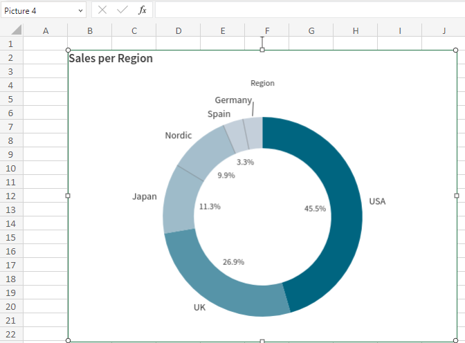
You can add a chart as an image to the Excel report template. When the report output is generated, an image of the chart is placed in the selected cell. The chart will use the data from the app's most recent reload.

A chart image is added as a placeholder image, representing a snapshot of what the chart looks like in the template creator's current session. This might include selections made in the app. It is important to remember that the selections in the chart snapshot are not included in the report output. Data reduction is instead controlled by report filters. For more information, see App selections and Working with report filters.

Do the following:

1. Click the icon on the top toolbar of the add-in.

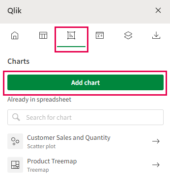
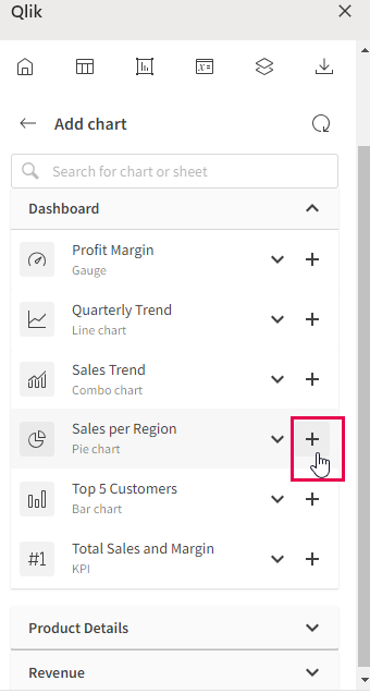
2. Click Add chart. A list of available sheets appears. Expand the sheet containing the chart you want to add, and click the icon to add it.

   

3. Expand the sheet containing the chart you want to add. You can search the chart's name to refine the list of sheets if needed.

4. Click the icon to add the chart.

   You can preview the chart directly in the add-in before adding it by clicking the chart's name.

   

5. The chart is added, and the settings page for the image appears. It is recommended to provide a unique Name to the table so you can identify it in the add-in if you later need to change its settings.

   Change the size of the image as you normally do with Excel images. Use the Zoom setting in the add-in as needed.

   

Revisit any chart you have added at any point for modifications to its configuration, to locate it in the workbook, or to add another instance of it to the workbook. Click the icon in the add-in to open the Charts landing page, and click to navigate to the cell where it is inserted. Adjust any settings as needed in the add-in.