
Applying the structured framework: Customer churn example
This example will walk you through the process of defining a machine learning question step by step. You will learn how to combine business knowledge with the framework of event trigger, target, prediction point, and features to structure a well-defined question.
The starting point is the business case "Will a customer churn?". By using the structured framework, we will boil this down to something more specific that can be predicted by a machine learning algorithm.
Event trigger
The event trigger is an action or event that triggers the creation of a new prediction. We identify our event trigger as "a customer has signed up for a subscription". This is represented in the data as a new customer is created. We want to predict at the customer level whether they will churn, so each row needs to represent a single customer.
Using our business knowledge and confirming by checking the data, we know that churn is highest among our new customers. We therefore decide to focus on new customers specifically. The event trigger is that a new customer signs up and we can think of each customer as having an individual time line starting the day they subscribe.
The event trigger is when a new customer subscribes. The horizontal line represents the number of days since subscribing.

Target
The target is the result we are trying to predict. We want to predict churn, so we know that our general target is "Will a customer churn?". But we need to be more specific to create a quality machine learning model. To start with, we decide that "churn" means that a customer calls us to cancel their subscription.
The target outcome is when a customer calls to cancel their subscription.

Next, we decide the time frame (the horizon) in which that cancellation call has to be made. When looking at multiple customers who have canceled, we see that the time line is not consistent. Some customers cancel after 45 days and others not until much later at 110 days.
Days since subscribing until the customer calls to cancel their subscription. Each line represents a different customer.

We have a 90-day free trial program and know that a lot of customers churn from the trial. Based on this business context, our initial thought is to use a horizon of 90 days. By predicting who is expected to cancel, we plan to reach out to those customers ahead of time and offer incentives (such as discounts or additional subscription features) to encourage them to stay.
A histogram of how many days after sign-up customers have canceled confirms our business intuition. In the figure we can see data for all customers who have churned in the last three years.
The distribution of cancellation calls over the number of days since subscribing. Most of the cancellations happen around 90 days after a customer subscribes.

Choosing a 90-day horizon seems like a good place to start. However, when we draw that horizon on our histogram we realize that there are a lot of customers who continue to churn for a few days after the 90-day trial period. The reason might be that they see their credit card get charged or get a notice that their payment method was declined a few days later and only then call in to cancel their subscription.
A horizon at 90 days after subscribing

Because we want to include these customers as "churned" in our model, we decide that it makes more sense to use 110 days as our target horizon. By using 110 days we capture most customers whose churn is likely related to the free trial program.
A horizon at 110 days after subscribing

Now that we have defined our target, we can determine where the data is stored and how it needs to be cleaned up to build the target column in the dataset. In this example we do the following:
-
Pull the customer status from Salesforce.
-
Extract status, customer created date, and customer cancellation date:
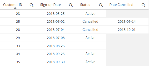
-
Clean and transform the extracted data into the target column:
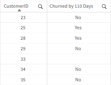
We have now defined our event trigger (a new customer signed up) and our target (the customer called to cancel their subscription within 110 days of signing up). They are illustrated on the timeline in the figure.
The event trigger is when a new customer signs up (1), the target outcome is when the customer calls to cancel (2), and the target horizon is 110 days after subscribing (3).

Prediction point
The prediction point is the designated time when you stop collecting data for features and predict the target for each row. The prediction point can fall anywhere between the event trigger (the day of subscription sign-up) and the target horizon (day 110 after sign-up). To pick a starting point we can think about the action we want to take.
In our example, maybe the customer support team has asked for 30 days to reach out to customers with retention offers once customers have been predicted to churn. This means that, at the very latest, we would want to predict 30 days before the target horizon, that is, by day 80.
The prediction point (2) is set at day 80, between the event trigger (1) and the target horizon (3).

Choosing day 80 as our prediction point would give us 80 days to collect data about new customers as they come in. This time frame between the event trigger and the prediction point is called the data accumulation window. Data collected during the data accumulation window is used to generate features.
The data accumulation window is the time between the event trigger and the prediction point.

Using day 80 as the prediction point leaves a 30-day action window, which is the time between the prediction point and the target horizon. This is the 30-day window the customer support team requested to reach out to customers.
The action window is the time between the prediction point and the target horizon.

In addition to thinking about the minimum action window required to take action on the predictions, we also need to look at the histogram of days until churn. Applying the day 80 prediction point, we would get the following:
The distribution of cancellation calls with the data accumulation window and the action window.

Looking at this histogram we realize that using a day 80 prediction point fails to maximize business value. Although 80 days’ worth of data helps to increase the accuracy of the model, it comes at a high cost for actionability:
-
First, a lot of customers have already churned by day 80, so they will have churned during the data accumulation window—before we are even making any predictions. This also means we would not want to include them in our training dataset because we would know the outcome prior to making the prediction.
-
Second, a lot of customers churn around day 80 to 90, so the customer success team would not have the full 30 days to reach out to those customers.
Customers who canceled their subscriptions before the prediction point will not be included in the training data.

Moving the prediction point to day 60 provides a better balance between accuracy and actionability. We still have 60 days to collect data to use for features in our model, but we are now predicting early enough that the customer success team has 30 days to reach out to most of the customers that we predict will churn. By reducing the data accumulation window, we can expect a small decrease in model accuracy, but a much more actionable prediction.
Moving the prediction point to day 60 shortens the data accumulation window but gives us a longer action window. It excludes fewer customers from the training data.

Features
With the event trigger, target and prediction point defined, we are ready to add the final part to our dataset: the features. Features are the known attributes, or observations, for each row of data in the training dataset from which the machine learning algorithms learn general patterns. The algorithms then use the features in order make predictions when presented with a new row of data in the apply dataset.
Think of features as your hypotheses that is based on business knowledge about what influences the outcome. In our example, some features could be customer location, lead source, sign-up month, number of logins, or number of active users.
There are two categories of features:
-
Fixed features are the most straight-forward because they do not change over time. In our example, customer location (at sign-up), lead source, and sign-up month are all considered fixed features. They are known as soon as a customer signs up (right at the event trigger) and no matter where we put our prediction point they will be both known and constant.
-
Window-dependent features are slightly more complicated. These are the features that are collected based on information collected between the event trigger and the prediction point. It's important to make sure that you are only using data that would be known in time, otherwise the model might have data leakage. (For more information, see Data leakage.)
A simple model might only use information known at day 0, that is, only fixed features. This would give a prediction point at day 0, as shown in the figure.
With a prediction point at day 0, we have 0 days to collect data and we can only use fixed features that are known at day 0. The action window is the full 110 days.

The resulting dataset would look something like this:
Training data with only fixed features

However, we might also want to use data collected once the customer has subscribed, as in our example with the prediction point at day 60.
The prediction point at day 60 gives us 60 days to collect data and 50 days to take action.
Now we can use information collected over the first 60 days after a customer signs up in order to add window-dependent features to our model. Our dataset for this model might look like the following table—now including the window-dependent features Logins First 60 Days and Active Users at 60 days.
Sample data with window-dependent features

Note that in this example, the features reflect the entire data accumulation window. They can also be smaller. For example, we could measure logins the first 10 days or logins day 30-60, as long as the features don't include any information past the prediction point.
Window-dependent features can be more complicated to collect because they require dates and need extra effort to ensure that they fall within the data accumulation window to avoid data leakage. But they can also be some of the most powerful features because they can reflect information collected much closer to the time of prediction.
The resulting machine learning question
We started with the simple use case "Will a customer churn?". We then defined our event trigger as "A new customer signs up" because we wanted to make predictions at the individual customer level.
We defined our target with a specific outcome—"Customer called to cancel their subscription (Yes or No)"—and set the horizon to 110 days because that is the time by which most of our trial customers have canceled.
Looking at a histogram of how many days after sign-up customers called to cancel over the past three years, we decided on a prediction point of 60 days after sign-up. This would give us 60 days to collect information (the data accumulation window) before making our prediction, but still give the customer support team time to take action on the predictions in order to reduce churn.
Finally, we gathered data on customers that would be available prior to day 60 to generate features.
Our resulting machine learning question is: "After the first 60 days of activity, will a customer call to cancel by day 110?"
And the dataset, which is now ready to be used for automated machine learning, looks like the table below. Location, Lead Source, Month Joined, and Subscription Amount are fixed features, Logins First 60 Days and Active Users at 60 Days are window-dependent features and Churned by 110 Days is the target column.
Sample data with fixed features (1), window-dependent features (2), and target (3)
