Imputation of nulls
Too many missing values could negatively impact the quality of your machine learning model. Imputation is the practice of filling missing values, known as null values. There could be many reasons for missing data such as a database error, a user who doesn’t fill out a part of a form, or maybe you start to collect new data and older records in the dataset don’t have the new data point.
It is important to understand the effects that imputation could possibly have on the data. Imputation retains the predictive power of the row or column, but it also has the potential to create patterns that didn’t previously exist or add noise to a pattern that did exist. This reduces the validity of the data.
You might want to review your data collection practices to ensure data completion and to implement new processes as needed. If you want to keep the representation of an empty value, you could fill in nulls with a value such as "other" or "unknown".
Null imputation during automatic preprocessing
In Qlik Predict, automatic data preprocessing uses null imputation to prepare your dataset for training. During the automatic data preprocessing, null values are handled by excluding columns missing more than 50 percent of the values and by imputing missing values. Missing values in categorical features are imputed with the value "other" and missing values in numeric features are imputed with the mean.
Additional considerations apply for auto-engineered features, time-aware training, and time series experiments.
For more information about preprocessing, see Automatic data preparation and transformation.
Auto-engineered features
With automatic feature engineering, Qlik Predict creates new features from existing parent features. For auto-engineered features, null imputation is performed as follows:
-
If you include auto-engineered date features in the training, the null imputation process for these features is the same as it is for numeric features.
-
If you use instead use the parent date features, the null imputation process is the same as it is for categorical features.
-
For categorical features that are treated as free text, null imputation is the same as it is for categorical features.
Time-aware training
If time-aware training is turned on, null imputation is performed as follows:
-
Any rows in the training dataset that have a null value for the selected date index are dropped during preprocessing. These rows are not used to train the models.
-
For numeric features, null imputation is performed with linear interpolation. Linear interpolation is also used for auto-engineered date features.
-
For categorical features, the null imputation process is the same as when you are not using time-aware training.
-
If you use date features without automatic feature engineering, the null imputation process is the same as it is for categorical features.
-
For categorical features that are treated as free text, null imputation is the same as it is for categorical features.
For more information about time-aware training, see Creating time-aware models.
Time series experiments
For time series experiments, null imputation is performed as follows:
-
For records where a group or date index value is missing, the entire record is dropped and its values replaced with imputed values.
-
In datasets for time series experiments, the date index column can also have gaps in its time steps. In these cases, imputation is also performed to add these entire missing records to the dataset.
How does imputation work
The following methods are common practices for imputation of nulls.
Numerical values
A good default is to impute the mean value. If the missing values are normally distributed, it is like adding weight to the center of a seesaw—it doesn’t affect the weight to either side. However, you should always consider what the value is trying to represent. For example, if some of the values for sales price are null in your sales data, is it caused by a database error or did the buyer use a coupon as payment? Would a 0, or some other value than the mean, make more sense?
Categorical values
A good default for categorical values is to add another category and call it "Other", "Unknown", or even "Missing". This category can hold the additional variance if the missing values are randomly distributed, or gain in feature importance if there is a meaningful relationship between missing that value and the target value.
A fallback is to impute the average in the form of the mode. As with numerical values, it is always important to consider both what the value is actually trying to represent and why the value might be missing. If you know that most of the missing values are probably the mode, you can impute with the mode. If it’s not known, or there is uncertainty, you can impute the categorical value with a filler text that is a new unique value to the dataset.
Effects of imputing numerical values
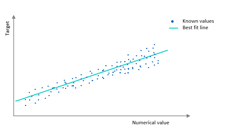
Numerical imputation 1 shows a scatter plot with a best fit line. We have a numerical value along the category (x) axis and a target value along the value (y) axis. It appears to be a good fit, but it is only taking into account points of data where x is known.
Numerical imputation 1: Plot of known values with a best fit line

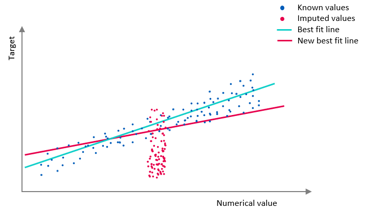
In Numerical imputation 2, we have imputed the mean value. However, the missing values don't seem to be random. This ends up skewing the line of best fit and adds noise, thereby reducing the overall accuracy of the model.
Numerical imputation 2: Plot of known values and imputed mean values. The imputed values are not randomly distributed and there is a new best fit line.

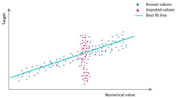
The chart in Numerical imputation 3 shows what it would look like if we impute the mean when the missing values are randomly distributed. In other words, when there is no additional knowledge to be gained by knowing if the value was present or missing. When the missing values are randomly distributed, it does not change the line of best fit. If we had imputed 0 instead of the mean value, it would have changed the line of best fit in a similar way as in Numerical imputation 2.
Numerical imputation 3: Plot of known values and randomly distributed imputed values. The best fit line has not changed.

Example: Loan qualification
A real world example of would be if x was the annual income and y the amount someone would be able to qualify for on a loan. We would expect a relationship where the more money someone makes, the more money they can borrow. The pattern would be similar to Numerical imputation 1 above.
Imagine that people who make less money are less likely to submit their annual income. In this case, the x value is missing due to a specific reason. Imputing the mean for those values would skew the results of the model. The result would be something like Numerical imputation 2.
Now, consider that some records in the database were randomly deleted. The records contained data on how much money some people make, but not the record for the person. So the x-value is randomly null. That effect is pictured in Numerical imputation 3 and is a case where we can safely impute the missing value.
Another thing to consider is: what if 0 was imputed instead of the mean? In the loan qualification example, it is probably not an accurate representation to say that someone makes 0 dollars annually. It would skew the model similarly to Numerical imputation 2.
Effects of imputing categorical values
In the numerical case above, we used the mean to impute missing values. A simple method for categorical values is to take the mode, which is the most frequently occurring value. Some of the challenges present in imputing the mode are the same as in imputing the mean for a numerical value.
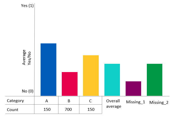
In the chart below, there is a pattern to the missing values in Missing_1 in relation to the target, whereas Missing_2 is randomly distributed. We can see this because Missing_2 matches the overall average target value. Missing_1 is similar to Numerical imputation 2 and Missing_2 is similar to Numerical imputation 3.
Categorical imputation: The columns Missing_1 and Missing_2 are examples of missing values with and without a pattern.

The difference to the numerical example is that in this case Missing_1 and Missing_2 both skew the pattern recognition. It is only being skewed for a subset of the data, category B, which would be the imputed value if imputing with the mode because it is the largest category.
Skewing the relationship between a single value and the target value is not the only risk in imputation, but it is among the most common and easiest to evaluate. Other risks tend to simply add noise and reduce accuracy. Fortunately, the risk of skewing can be greatly mitigated by dropping dimensions that are relatively sparse. There is often debate about exactly what sparsity levels to allow in a column or a row, but it is less often debated that imputing values has the potential to distort the data in a way that it is no longer representative of what the data is trying to describe.
