
Excel reports with levels
You can use levels to group the data in your report by a dimension. Levels can be applied to tables and images.
Levels cycle report elements through the values of a field. The results for each level field value are displayed in order.
For example, you have a Qlik Sense app with a table listing each product you have sold in a year. The table is very long and does not fit well on the Excel sheet. You can add that table to a Qlik NPrinting report, and add a level for Product Category. Your generated report will have a different table for each value of Product Category, instead of one large table.
You can create complex hierarchies with nested levels. For example, you can create a year > category hierarchy to generate a report with sales for each product category for each year. You can nest as many levels as you want, but performance will decrease with each addition of a level.
You can use QlikView objects that have calculated dimensions or null values as levels. However, you cannot nest other objects inside them, except for fields from that sheet object. Qlik Sense visualizations with calculated dimensions cannot be used as levels.
Performance
Report and preview generation slows down with the addition of levels. Charts and tables are extracted separately for each value in the level field, so the number of exported objects can increase significantly.
Rules
Each level has an opening tag and a closing tag. These tags do not have to be in the same row or column, but there are some rules for how you can place them:
- The opening tag must be in a row above all the rows containing tags to be cycled. It must also be in a column to the left of, or the same as, any column containing tags to be cycled in the level.
- The closing tag must be in a row below all rows containing tags to be cycled.
- Rows containing level tags will not be present in the report. You should not put content in the same row as a level tag.
- Any empty rows included in the level range will be present in the report.
- You can verify the level range by clicking on the level node. The level range will be outlined and highlighted.
If you drag and drop a level tag into the wrong cell, you can cut and paste it somewhere else.
What you will do
In this tutorial, you create a report where the QlikView objects inserted between the level opening and closing tags are organized by two fields. You will:
- Embed one object as a table and one as an image.
- Add two fields as levels so that the Excel report presents three tiers of information.
- Add titles and headings.
This tutorial uses QlikView data that can be found in Sample files. You can also use your own QlikView or Qlik Sense data.
Adding an image and a table
Do the following:
- Create a new Excel report, or open an existing template.
- Right-click the Images node, and select Add objects.
-
Select Top 5 Salesmen from the objects list. Click OK.
Under the Images node, you will see CH319 - Top 5 Salesmen.
- Right-click the Tables node, and select Add objects.
-
Select Top 5 Customers. Click OK.
Under the Tables node, you will see CH318 - Top 5 Customers.
-
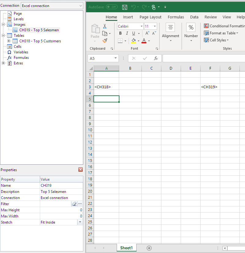
Drag the CH318 - Top 5 Customers and CH319 - Top 5 Salesmen tokens onto empty cells in the same row.
Make sure there are three or four empty columns between them.
Adding the first level
Levels have opening and closing tags that your table and image tags need to sit inside. The opening tag must be in a row above the objects you want to cycle. The closing tag must be in a row below.
Do the following:
- Right-click the Levels node, and select Add levels.
- Select Year from the list. Click OK.
- Right-click the Levels node, and select Add levels.
- Select CategoryName. Click OK.
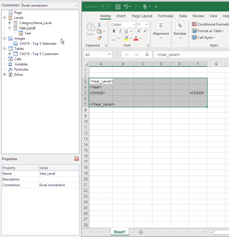
- From the left pane, drag and drop the Year_Level token onto empty cells in the worksheet.
-
Move the <Year_Level> opening tag so it is in a row above all rows you want to include in the cycle.
It must also be in the same column as (or a column to the left of) all columns to be repeated in the cycle.
Empty rows included in the level range will be reproduced in the cycle.
-
The closing level tag </Year_Level> must be in a row below any rows you want to include in the level cycle.
You can verify which elements are included in the cycle by clicking on the Year_Level node in the left pane. This highlights the level range.
-
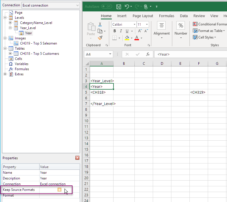
You can include a dynamic, customizable heading for the level cycle. Expand the Year_Level node and click on the Year node token. In the Properties pane, clear the Keep Source Formats check box.
-
Drag the Year tag onto the Excel sheet, in a row below the <Year_Level> opening tag. You can format the Year tag the same way you would format any text in Excel.
Adding the second level
We are going to add a second level, CategoryName_Level, above Year_Level. This means that your report will be organized by product category, and then year.
Example: Product category > Year
- Baby clothes
- 2012
- 2013
- 2014
- Men's shoes
- 2012
- 2013
- 2014
You can also do the opposite, and nest CategoryName_Level inside year.
Example: Year > Product category
- 2012
- Baby clothes
- Men's shoes
- 2013
- Baby clothes
- Men's shoes
- 2014
- Baby clothes
- Men's shoes
Do the following:
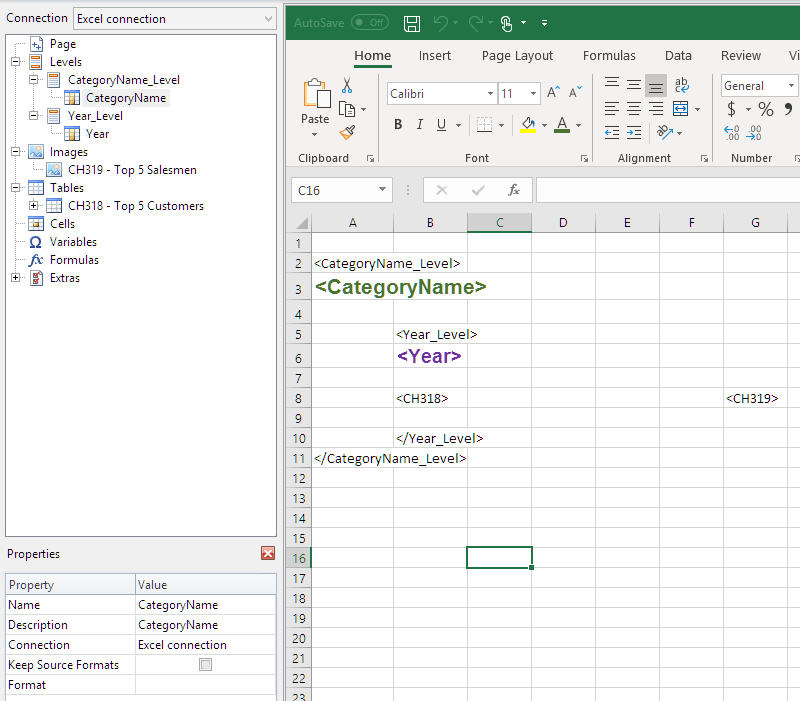
- From the left pane, drag the CategoryName_Level token onto an empty part of the sheet.
-
Position the <CategoryName_Level>opening tag above the <Year_Level> token.
It must also be in the same column or a column to the left of <Year_Level>. Add a new column on the left if you need.
- Place the </CategoryName_Level> closing tag in a row below all other objects.
-
If you want to include a dynamic CategoryName heading: in the left pane, expand the CategoryName_Level node in the left pane by clicking on the +.
-
Drag and drop the CategoryName node token into the row directly beneath the <CategoryName_Level>opening tag.
You can format the tag the same way you would format any text in Excel.
Previewing the report
Do the following:
-
Click Preview.
Excel launches and displays your report.
-
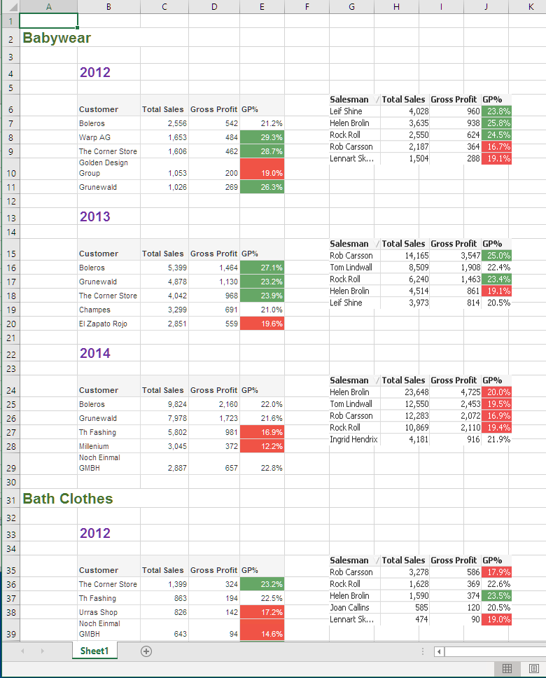
You will have a report organized by your first level, and then your second level.
- Click Save and Close to save the template, and close the Template Editor.