
Excel reports with nested levels and subtotals
You can nest levels to create a hierarchy and use Excel formulas to make calculations.
For example, you can create a year > category hierarchy to obtain a report with sales for each product category for each year. You can add summary formulas and labels to each level of the report to show which values are displayed in that level. To learn about levels, see: Excel reports with levels.
You can use QlikView objects that have calculated dimensions or null values as levels. However, you cannot nest other objects inside them, except for fields from that sheet object. Qlik Sense visualizations with calculated dimensions cannot be used as levels.
What you will do
In this tutorial, the QlikView objects inserted between the level opening and closing tags will be sub-divided in the final report.
You will:
- Create a custom table by adding two table columns.
- Add two fields as levels so that the Excel report presents three tiers of information.
- Add SUM formulas so your tables have totals and subtotals.
- Customize SUM formulas using Excel formatting. This tutorial has suggested formatting, but you can customize your design to your specifications.
This tutorial uses QlikView data that can be found in Sample files. You can also use your own QlikView or Qlik Sense data.
Creating a new Excel report
Do the following:
- Select Reports in the Qlik NPrinting main menu, and then click Create report.
- Enter a Title for the report. Report with nested levels and subtotals.
- Select Excel from the Type drop-down list.
- Select an app from the App drop-down list.
- Click Create to create the report.
- Click Edit template to open the Template Editor.
Choosing levels and table objects
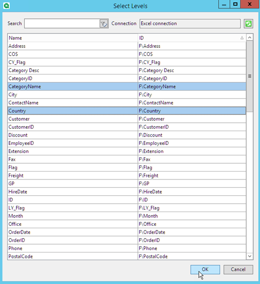
- Right-click the Levels node, and select Add levels.
-
Click the objects that you want to add. For example, add the Country and CategoryName fields.
You can hold down CTRL or Shift to select multiple items.
-
Click OK.
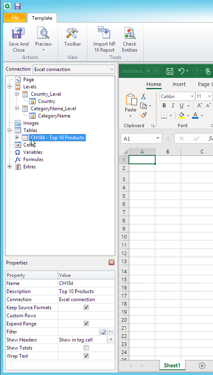
- Right-click the Tables node, and select Add objects.
- Click the object that you want to add. For example, select Top 10 Products.
-
Click OK.
Adding the table
You can add the entire table object to the template. In this example, you will only add two columns.
Do the following:
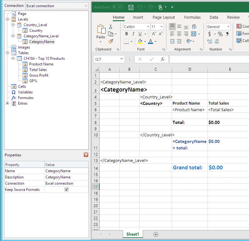
- Under the Tables node, expand the Top 10 Products node.
- Click on Total Sales. In the Properties pane, clear Keep Source Formats.
- Repeat for ProductName.
-
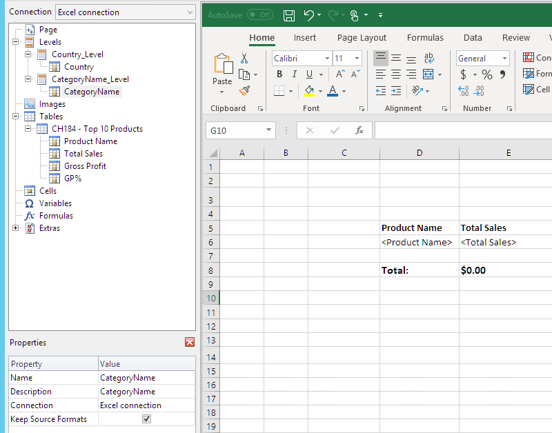
Drag the ProductName and Total Sales nodes onto empty cells in the template.
For example, cells D6 and E6.
- Click on <Total Sales>, and format as currency.
-
In cell E8, enter the Excel formula: =SUM(E6:E7).
This formula includes an empty row, so Qlik NPrinting will add rows as necessary to contain all values.
- In cell D8, type Total:.
-
Format cell E8 using Excel formatting.
For example:
- 12px bold font
- Right justified alignment
- Custom = Accounting with no digits to the right of the decimal point.
Adding the first level
Do the following:
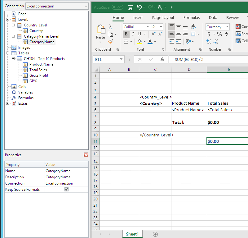
- Drag the Country_Level node onto cell C4.
- Move the </Country_Level> closing tag down to C10, so that Country Level includes the cell containing the SUM, and an empty row.
- Click + to expand the Country_Level node.
-
Drag the Country node token onto cell C6.
This adds a dynamic title.
- Format cell C6 to 12px and bold.
-
In cell E11, enter the formula: =SUM(E6:E11)/2.
The sum is divided by two because the SUM function will include all values, including the sum of those values that are in cell E8.
- Format cell E11 to:
- 12px bold font
- Right justified alignment
- Custom = Accounting with no digits to the right of the decimal point.
Adding the second level
Do the following:
- Drag the CategoryName_Level node token onto cell A2.
- Drag the </CategoryName_Level> closing tag down to A14.
- Click + to expand the CategoryName_Level node.
-
Drag the CategoryName node token onto cell B3.
This adds a dynamic title.
- Format cell B3 to 16px bold font.
- Drag a second CategoryName node to cell D11. Double-click this cell and add the word "total", so the cell displays <CategoryName> total:.
- In cell D14, type in Grand total:.
-
In cell E14, enter the formula: =SUM(E2:E14)/3
The sum is divided by three because the SUM function will add all the values, including the subtotals in cells E8 and E11.
- Format cell E14 to:
- 14px bold font
- Right justified alignment
- Custom = Accounting with no digits to the right of the decimal point.
Previewing the report
Do the following:
-
Click Preview.
Excel launches and displays your report.
-
You will have a report organized by your first level, and then your second level.
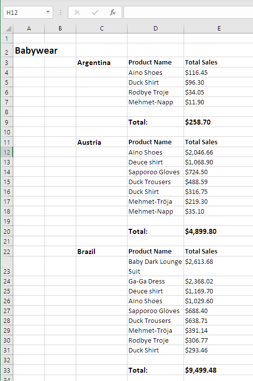
-
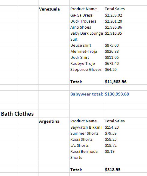
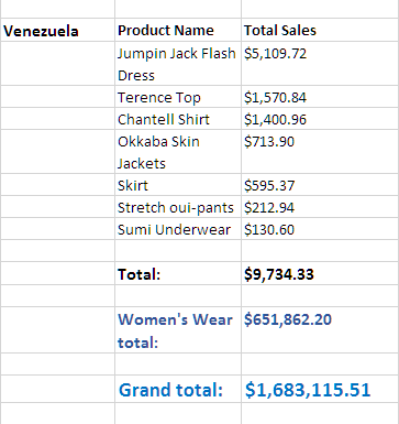
Each table will have a total underneath. Each category will have a total with a dynamic label.
-
At the bottom, there will be a grand total of all products from all countries.
- Click Save and Close to save the template, and close the Template Editor.