
Creating Excel reports
In this tutorial, you will create a new Excel report template with two tables and an image. You will use the Page feature to produce a new worksheet for each value of a field.
What you will do
You will:
- Create a new Excel report template.
- Add a table object.
- Create a custom table column by column.
- Add an object as an image.
- Use the Page feature to generate a new worksheet for each different sales office.
This tutorial uses QlikView data that can be found in Sample files. You can also use your own QlikView or Qlik Sense data.
Creating a new Excel report template
Do the following:
- Select Reports in the Qlik NPrinting main menu, and then click Create report.
- Enter a Title for the report.
- Select Excel from the Type drop-down list.
- Select an app from the App drop-down list.
-
Select a Template from the options available:
- Empty template - uses an empty template
-
Default template - use the default template (only available if a default template has been set in Report settings.
- Custom - Choose a file to use as a template.
- Leave the Enabled check box selected. If you clear it, the report will be saved, but ignored by the scheduler.
- Click Create to create the report.
- Click Edit template to open the Template Editor.
Adding a table
Do the following:
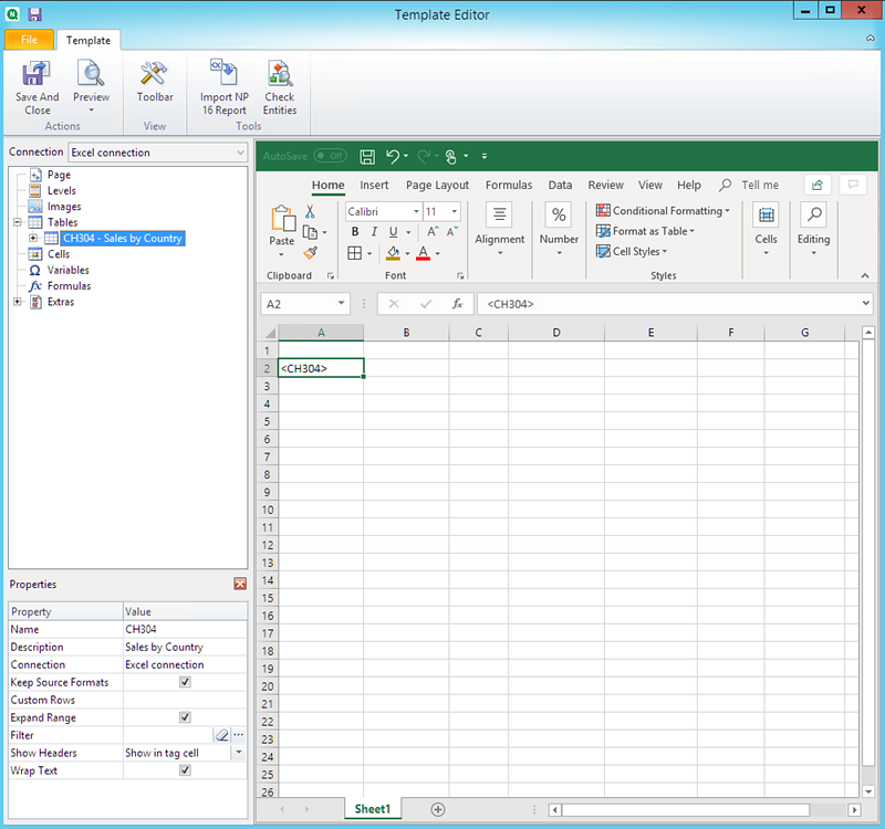
- Right-click the Tables node, and select Add objects.
- Select Sales by Country from the objects list. Click OK.
-
Drag and drop the CH304 - Sales by Country tag onto an empty cell.
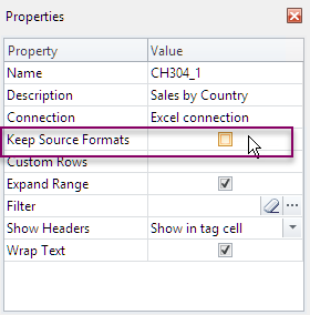
Customize the formatting on an entire table
This causes the contents of all cells in all columns of the table to be exported from QlikView or Qlik Sense without formatting. You can apply new formatting using the Excel ribbon.
Do the following:
- On the left-hand pane, select the table you want to customize.
- Go to the Properties pane.
-
Clear the Keep Source Formats check box.
-
Use the Excel ribbon to customize the table.
For example, change font size or color.
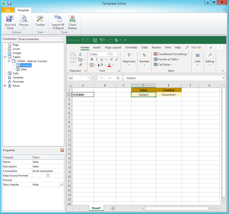
Adding a table column by column
You can create a custom table by adding columns individually. They do not have to be in the same order as the original Qlik Sense or QlikView table.
Do the following:
-
Expand the CH304 - Sales by Country node.
Information noteYou can only expand the node to reveal column nodes if the object is a straight table or table box. If you do not see the +, you added a pivot table or a straight table with calculated columns. -
Drag and drop the column tags into cells one at a time.
This creates a tags for each selected column with its title as a text cell that you can format.
You can move the tags in the Excel template to obtain the column order you prefer.
Customize formatting on specific columns in a table
If you want to keep the source formatting for the majority of columns, leave the Keep Source Formats box selected for the table as a whole. You can disable Keep Source Formats on individual columns. This causes the content of all cells in the selected column to be exported from QlikView or Qlik Sense without formatting. You can apply formatting using the Excel ribbon.
Do the following:
-
Expand the table node by clicking the + on the left.
- Select the column that you want to customize.
- In the Properties pane, clear the Keep Source Formats check box.
-
Select the column in the template, and then apply formatting as desired.
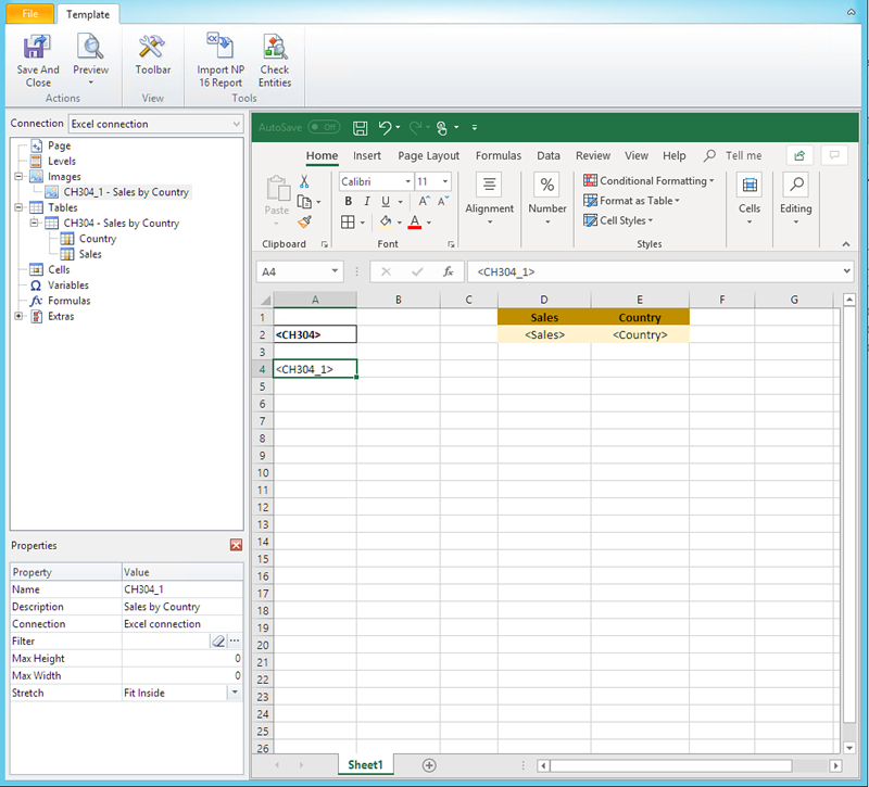
Adding an image
Do the following:
- Right-click the Images node, and select Add objects.
- Select Sales by Country from the objects list. Click OK.
-
Drag and drop the CH304_1 - Sales by Country tags onto any cell below the tables.
Previewing the report
Do the following:
-
Click Preview.
Excel launches and displays your report.
-
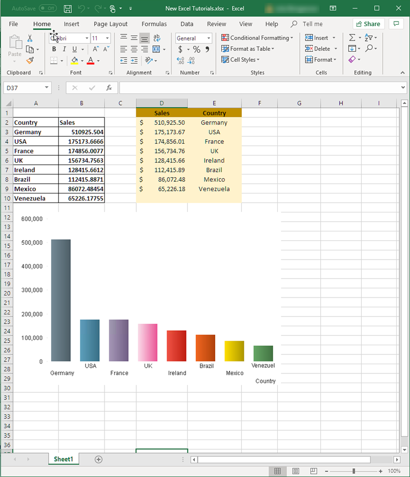
You will see an Excel report with one sheet. That sheet will have the same Qlik object as an image, a table, and a table added column by column.
- Close the preview window.
Applying Pages
The Pages node lets you produce a report with a separate worksheet for each value of a field. For example, a different worksheet for each sales office.
Do the following:
- Right-click the Page node icon in the left pane.
- Select Add page to current sheet.
- Select SalesOffice from the list. Click OK.
- Click the + on the left to expand the SalesOffice page node.
-
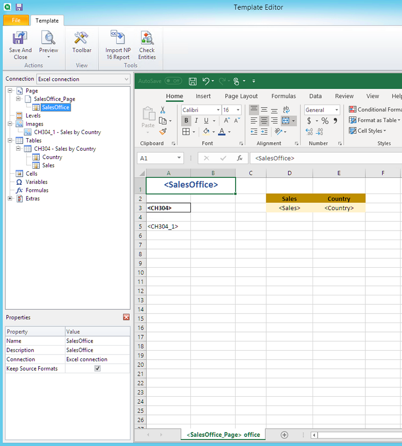
Drag the SalesOffice node tag onto a cell in the template.
You can format the cell using Excel formatting features.
-
The worksheet name changes to <SalesOffice_Page> on the bottom tab. When the report is generated, this will be replaced with the related value of each worksheet.
You can edit the worksheet name by adding text. For example: <SalesOffice_Page> office.
Your report will now be produced with a different worksheet for each sales office.
Preview and save
Do the following:
- Click Preview.
-
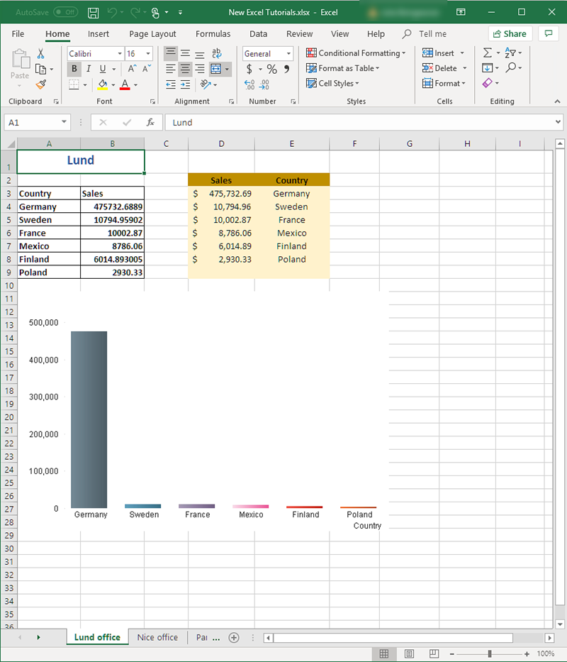
You will see a report with sales office as a title, two tables, and an image. There are now several worksheet tabs, one for each office.
- Click Save and Close to save the template and close the Template Editor.